 |
For our lab course we need a system language for describing 1-safe Petri nets of
a moderate size, say at most 100 nodes.
The intended users are students who need to code nets directly in this
language, i.e. we do not intend to provide a graphical editor.
The students will only be familiar with low-level nets.
Generally speaking, data needed to define 1-safe low level Petri nets
are details on places, transitions, arcs and an initial marking.
Therefore we define our language as follows:
SENIL

@trans

P1, ... -> T1{@label, ... } -> P3, ...

# T1 -> P1, ...

P1, ... -> T1 #

@place

T1, ... -> P1 -> T2, ...

# P1 -> T1, ...

T1, ... -> P1 #

@marking

P1, P2, P3, ...

@partition

P1, P2, P4, ...

P3, P5, P6, ...

.

.

.
- A net must start with the keyword
SENIL.
-
One can describe Petri nets from the
point of view of the transitions
by listing the presets and postsets of the transitions.
The special symbol
@trans signifies
the start of a block in which each line holds a
transition surrounded by arrows (->).
Each line begins with the list of places in the preset and
ends with the list of places belonging to the postset.
Empty presets or postsets are denoted by
# or '.'.
-
Alternatively you can list the presets and postsets of places behind the
special symbol
@place.
In these lines the place is denoted between arrows, and the transitions of the
preset and postset are before and behind it, respectively.
Note that the preset or postset, or both, can be empty, in which
case they must be replaced by # or
'.'.
- The places which are initially marked can be listed behind the
keyword
@marking.
- Some tools can make use of further informations regarding partitions.
Each line after the keyword
@partition defines a list of
places that form a partition.
- Sometimes it is very useful to furnish transitions or places with additional
information like labels etc. Each transition or place may be followed
by additional information enclosed in braces; different fields
can be separated by commas.
Each additional information must be
denoted by a special keyword. For example, the label of a transition
can be denoted by
T1 {@label a}.
The language is easily extensible because each additional
information needed in future works can be appended
by defining a new special keyword at the beginning of the new
information.
Example:
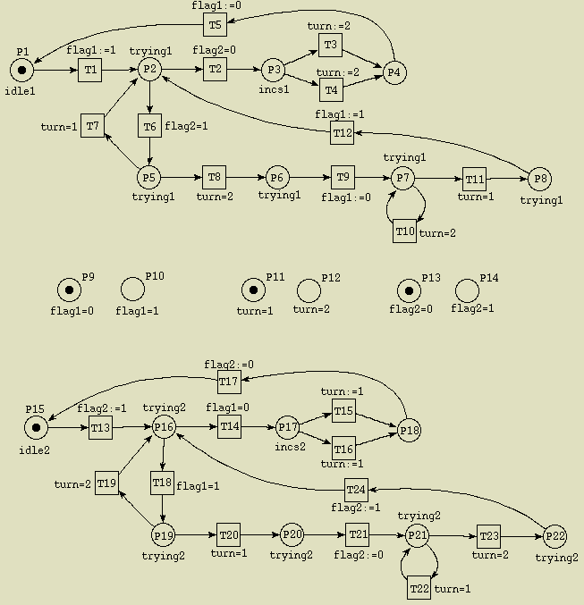
By means of Dekker's mutex algorithm we show how to model the algorithm in
SENIL. For that we need the algorithm described as a 1-safe Petri net.

Places P9 through P14 denote different values of the variables.
For example, if process 1
fires transition T1, then afterwards the value of variable flag1
should be set to 1. Moreover, we know that the value of flag1 is
0 before execution of T1. To model this behaviour correctly, we
have to draw edges from P9 to T1 and from T1 to
P10. Transition T2 should be fired only if process 1 stays in
state P2 (it is marked) and if the value of variable flag2 is
0 before execution of T2. So we have to draw an edge from
P13 to T2. Also, we must draw an edge from T2 to
P13 because the value of flag2 will not be changed during
execution of T2.
For the sake of clarity all edges
connecting places P9 through P14 with transitions are omitted.
See here for the Petri net with all edges.
Now, it is an easy task to model Dekker's mutex algorithm
in SENIL:
First, for the sake of clarity, we only want to give labels to all places and
transitions. Therefore, all presets and postsets are empty (denoted by
#). Then we define the Petri net from the point of view of
the transitions by describing their presets and postsets. For example, the
line P1, P9 -> T1 -> P2, P10 means that there are arcs
going from places P1 and P9 to transition
T1 and from transition T1 to places P2
and P10. At the end, all initially marked places are listed
(P1, P9, P11, P13,
P15).
SENIL
@place
# P1 { @label "idle1" } #

# P2 { @label "trying1" } #

# P3 { @label "incs1" } #

# P5 { @label"trying1" } #

# P6 { @label "trying1" } #

# P7 { @label "trying1" } #

# P8 { @label "trying1" } #

# P9 { @label "flag1=0" } #

# P10 { @label "flag1=1" } #

# P11 { @label "turn=1" } #

# P12 { @label "turn=2" } #

# P13 { @label "flag2=0" } #

# P14 { @label "flag2=1" } #

# P15 { @label "idle2" } #

# P16 { @label "trying2" } #

# P17 { @label "incs2" } #

# P19 { @label "trying2" } #

# P20 { @label "trying2" } #

# P21 { @label "trying2" } #

# P22 { @label "trying2" } #

@trans

# T1 { @label "flag1:=1" } #

# T2 { @label "flag2=0" } #

# T3 { @label "turn:=2" } #

# T4 { @label "turn:=2" } #

# T5 { @label "flag1:=0" } #

# T6 { @label "flag2=1" } #

# T7 { @label "turn=1" } #

# T8 { @label "turn=2" } #

# T9 { @label "flag1:=0" } #

# T10 { @label "turn=2" } #

# T11 { @label "turn=1" } #

# T12 { @label "flag1:=1" } #

# T13 { @label "flag2:=1" } #

# T14 { @label "flag1=0" } #

# T15 { @label "turn:=1" } #

# T16 { @label "turn:=1" } #

# T17 { @label "flag2:=0" } #

# T18 { @label "flag1=1" } #

# T19 { @label "turn=2" } #

# T20 { @label "turn=1" } #

# T21 { @label "flag2:=0" } #

# T22 { @label "turn=1" } #

# T23 { @label "turn=2" } #

# T24 { @label "flag2:=1" } #

P1, P9 -> T1 -> P2, P10

P2, P13 -> T2 -> P3, P13

P3, P11 -> T3 -> P4, P12

P3, P12 -> T4 -> P4, P12

P4, P10 -> T5 -> P1, P9

P2, P14 -> T6 -> P5, P14

P5, P11 -> T7 -> P2, P11

P5, P12 -> T8 -> P6, P12

P6, P10 -> T9 -> P7, P9

P7, P12 -> T10 -> P7, P12

P7, P11 -> T11 -> P8, P11

P8, P9 -> T12 -> P2, P10

P15, P13 -> T13 -> P16, P14

P16, P9 -> T14 -> P17, P9

P17, P12 -> T15 -> P18, P11

P17, P11 -> T16 -> P18, P11

P18, P14 -> T17 -> P15, P13

P16, P10 -> T18 -> P19, P10

P19, P12 -> T19 -> P16, P12

P19, P11 -> T20 -> P20, P11

P20, P14 -> T21 -> P21, P13

P21, P11 -> T22 -> P21, P11

P21, P12 -> T23 -> P22, P12

P22, P13 -> T24 -> P16, P14

@marking

P1, P9, P11, P13, P15
Atomic propositions can consist of ...
- Place names
A place name can be an atomic proposition, for example P1, P2,
P3.
- Place labels
One can use the label of a place as atomic proposition, for example
"incs1".
Labels must be typed in quotes.
|
|

